The Viewer

Lesson 6 of 6. The last one. The answer is on branch step-6-viewer of plesty-demo-pol-pl.

One curve told you the sweep was working. It did not tell you the emission sits at 779.7 nm, or that the line stays put while its brightness turns over — for that you need the spectra, and the spectra are the part of the measurement you have not touched yet: 1340 numbers a row, on a disk, in files the record only points at.

This lesson gets them onto the screen. Three views of the same run, side by side, and you write all three.

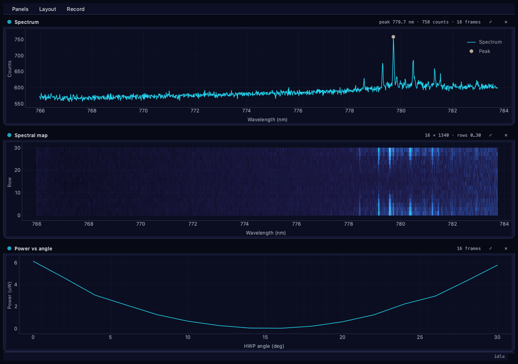
Lesson 5 gave you the contract and one view built on it. Nothing in this lesson is a new idea — it is the same input_schema, traces(), update() three more times, against data that happens to be arrays instead of scalars. The window at the end is twelve lines.

You added plesty-lib[gui] in lesson 5. The video at the end needs one more extra:

uv add "plesty-lib[gui,record]"

Open the frame

A record carries a path, not a spectrum. That is lesson 4's rule — blob data never crosses the network — and it means something has to open the file before any view can draw it. The format is the spectrometer's, so this is the one part of the lesson that is about a vendor rather than about PLESTY.

A new file, plesty/demo_pol_pl/frames.py:

"""Reading the spectrometer frames a run left on disk."""

from __future__ import annotations

import struct
import xml.etree.ElementTree as ET
from pathlib import Path

import numpy as np

#: Byte offset of the 64-bit pointer to the XML footer, in SPE v3.
FOOTER_POINTER = 678

#: Byte offset where the pixel block starts, in SPE v3.
DATA_OFFSET = 4100


def read_spe(path: str | Path) -> tuple[np.ndarray, np.ndarray]:
    """Read one SPE frame as a spectrum.

    Args:
        path: The frame file.

    Returns:
        The wavelength axis in nanometres (pixel indices when the file has no
        calibration) and the detector rows summed into one spectrum.

    Raises:
        ValueError: If the XML footer lacks the block that says how the pixel
            data is shaped.
    """
    raw = Path(path).read_bytes()
    footer = struct.unpack_from("<Q", raw, FOOTER_POINTER)[0]
    root = ET.fromstring(raw[footer:].decode("utf-8", errors="ignore"))
    ns = {"a": root.tag.split("}")[0].strip("{")}

    region = root.find(".//a:DataFormat/a:DataBlock/a:DataBlock", ns)
    if region is None:
        raise ValueError("SPE footer lacks the frame/region DataBlock structure.")
    width, height = int(region.get("width") or 0), int(region.get("height") or 0)
    counts = (
        np.frombuffer(raw, dtype=np.uint16, count=width * height, offset=DATA_OFFSET)
        .reshape(height, width)
        .sum(axis=0)
        .astype(float)
    )

    node = root.find(".//a:Calibrations//a:WavelengthMapping/a:Wavelength", ns)
    wavelength = (
        np.array([float(value) for value in node.text.split(",")])
        if node is not None and node.text
        else np.arange(width, dtype=float)
    )
    return wavelength, counts

An SPE v3 file is a fixed header, a block of unsigned 16-bit pixels, and an XML footer describing them. The two constants are where that structure is nailed down: a 64-bit pointer at byte 678 says where the footer starts, and the pixels always begin at byte 4100. The footer says how wide and how tall the readout was, and carries the wavelength of every pixel when the spectrometer was calibrated — which is the difference between a plot that reads in nanometres and one that reads in pixel numbers.

Summing the rows is a decision, not a formality: the detector read height rows and a spectrum is one. A different experiment might want them kept apart.

Check it against a frame your own run wrote:

uv run python -c "
from plesty.demo_pol_pl.frames import read_spe
wl, counts = read_spe('$RUN_DIR/raw/<one-of-the-files>.spe')
print('points:', counts.size)
print('range: %.1f - %.1f nm' % (wl[0], wl[-1]))
i = counts.argmax()
print('peak: %.1f nm, %.0f counts' % (wl[i], counts[i]))
"

points: 1340
range: 766.0 - 783.7 nm
peak: 779.7 nm, 755 counts

There is the number the introduction promised, out of your own parser.

Two views, one schema

Both spectra views consume the same thing, so they declare it once. In plesty/demo_pol_pl/monitors.py, below what lesson 5 left there:

SPECTRUM_CHANNELS = {
    "wavelength": {
        "dtype": "array_float",
        "unit": "nm",
        "description": "Wavelength axis of the detector row",
        "shape": [None],
    },
    "counts": {
        "dtype": "array_float",
        "unit": "counts",
        "description": "Detector counts of one acquisition",
        "shape": [None],
    },
    "row": {
        "dtype": "float",
        "unit": "deg",
        "description": "Plate angle this acquisition was taken at",
        "required": False,
    },
}

Three things here are new since lesson 5. array_float is an array channel rather than a scalar, and shape: [None] says one dimension of any length — the readout is 1340 bins today and something else on another grating. required: False marks row as a channel a view can do without: the map falls back to arrival order when nothing says where the acquisition sits in the sweep.

Sharing one schema between two monitors is what lets one mapper feed both. It is worth doing deliberately rather than by copy — the moment the two disagree, the mapper serves one of them and fails the other.

The spectrum

class SpectrumMonitor(Monitor):
    """The newest spectrum, with its peak marked."""

    title = "Spectrum"
    input_schema = SPECTRUM_CHANNELS

    def traces(self) -> list[TraceSpec]:
        """Declare the spectrum line and the marker sitting on its peak."""
        return [
            TraceSpec(
                "spectrum",
                "line",
                label="Spectrum",
                x_label="Wavelength (nm)",
                y_label="Counts",
                color="cyan",
            ),
            TraceSpec(
                "peak",
                "scatter",
                label="Peak",
                x_label="Wavelength (nm)",
                y_label="Counts",
                color="amber",
                width=9.0,
            ),
        ]

    def update(self, frame: Frame) -> dict[str, TraceData]:
        """Draw this acquisition, and put the marker on its brightest bin."""
        counts = np.asarray(frame["counts"], dtype=float)
        wavelength = np.asarray(frame["wavelength"], dtype=float)
        peak = int(np.argmax(counts))
        self._peak_nm, self._peak_counts = float(wavelength[peak]), float(counts[peak])
        return {
            "spectrum": TraceData(x=wavelength, y=counts),
            "peak": TraceData(x=[self._peak_nm], y=[self._peak_counts]),
        }

    def status(self) -> str:
        """Report the peak, so a drifting line shows without reading the plot."""
        if not self.count:
            return "waiting for the first spectrum"
        return f"peak {self._peak_nm:.1f} nm - {self._peak_counts:.0f} counts"

Two traces, one update. A view is not one curve — it is however many drawables it declared, filled in the same call. The second is a scatter of exactly one point, which is how you mark something on a plot: not a special annotation API, just a trace with one value in it. width=9.0 is its dot size.

No __init__, no reset. This view keeps only the newest acquisition, so there is nothing of its own to initialize and nothing to drop. Compare that with the map below, and with MalusMonitor — the obligation to override reset() comes with accumulating, and this class does not accumulate.

status() is the third thing a view can declare. The window puts it in the panel's title bar, and it is where a number belongs when reading it off the plot would be guesswork. A peak that walks from 779.7 to 779.2 over an hour is a drifting spectrometer, and you want that as digits.

The map

class WaterfallMonitor(Monitor):
    """Every spectrum of the run, stacked into one image."""

    title = "Spectral map"
    input_schema = SPECTRUM_CHANNELS

    def __init__(self, source: Optional[DataSource] = None, **params: Any) -> None:
        """Start with an empty map; the rows arrive one acquisition at a time."""
        super().__init__(source, **params)
        self._rows: list[np.ndarray] = []
        self._angles_deg: list[float] = []

    def traces(self) -> list[TraceSpec]:
        """Declare one image; its payload carries both axes."""
        return [
            TraceSpec(
                "map",
                "image",
                label="Spectral map",
                x_label="Wavelength (nm)",
                y_label="HWP angle (deg)",
                color="violet",
            )
        ]

    def update(self, frame: Frame) -> dict[str, TraceData]:
        """Append this acquisition as the next row of the map."""
        self._rows.append(np.asarray(frame["counts"], dtype=float))
        self._angles_deg.append(float(frame.get("row", len(self._rows))))
        return {
            "map": TraceData(
                image=np.vstack(self._rows),
                x=np.asarray(frame["wavelength"], dtype=float),
                y=np.asarray(self._angles_deg, dtype=float),
            )
        }

    def status(self) -> str:
        """Report how much of the sweep the map covers."""
        if not self._rows:
            return "waiting for the first spectrum"
        return (
            f"{len(self._rows)} x {self._rows[0].size} - "
            f"{self._angles_deg[0]:g}...{self._angles_deg[-1]:g} deg"
        )

    def reset(self) -> None:
        """Drop the accumulated map, then let the base class clear the view."""
        self._rows.clear()
        self._angles_deg.clear()
        super().reset()

image is the third trace kind, after line and scatter, and its payload carries image plus both coordinate axes. Handing over x and y is what makes the map read in nanometres and degrees rather than in pixel indices — the renderer scales the picture to the numbers you gave it. Leave them out and you get the same picture with meaningless axes.

This one accumulates, so it owns the two lists and the reset() override — exactly the shape MalusMonitor has. The frame.get("row", …) fallback is the required: False in the schema being honoured: no sweep position, rows numbered as they arrive.

One np.vstack per row is not a mistake worth fixing yet. Ninety-one rows of 1340 floats is under a megabyte, rebuilt twice a second. When a run is thousands of rows, that is where you would keep a preallocated array instead — and the change would be confined to this method, because nothing outside it knows how the map is stored.

One mapper, two views

The mapper is where the record's path becomes an array. It needs to be told how a path written by the acquiring host reads on this machine, so it takes that translation as an argument rather than assuming:

def spectra_row(locate: Callable[[str], Path]) -> FrameMapper:
    """Build the mapper both spectra views share.

    Args:
        locate: Turns the path as the record spells it into the path on this
            machine.

    Returns:
        A mapper that loads the frame a record points at.
    """

    def mapper(record: dict[str, Any]) -> Optional[dict[str, Any]]:
        if "data_file" not in record:
            return None
        try:
            wavelength, counts = read_spe(locate(record["data_file"]))
        except (OSError, ValueError):
            return None  # one unreadable frame costs one row, not the view
        return {"wavelength": wavelength, "counts": counts, "row": record["hwp_deg"]}

    return mapper

malus_row was a function; this is a function that builds one, because it needs configuring and a mapper takes only a record. That is the usual shape once a mapper knows anything about its surroundings.

The except is the interesting line. A frame can be missing, half-written, or on a share that just went away, and none of those should stop a window that is also drawing two other views of the same run. Returning None drops the row exactly as a bookkeeping record is dropped, and the next acquisition redraws. A view that raises here takes the whole shell down at three in the morning.

FrameMapper in that signature is the library's own name for the shape every mapper has — Callable[[dict[str, Any]], Optional[dict[str, Any]]], spelled out once in plesty/lib/monitor/sources.py and exported alongside the sources. It is the type RunSource(mapper=…) is annotated with, so a function that satisfies it is a function RunSource will take. malus_row from lesson 5 already matches it, without having said so.

Update the imports at the top of monitors.py for the two views and the mapper:

from pathlib import Path
from typing import Any, Callable, Optional

import numpy as np

from plesty.lib.monitor import DataSource, Frame, FrameMapper, Monitor, TraceData, TraceSpec

from .frames import read_spe

Dock them

plesty/demo_pol_pl/viz.py is the file you opened one panel with in lesson 5. Replace it with this — the whole thing:

"""The window that watches a polarization sweep."""

import sys
from typing import Iterator

from plesty.lib.experiment.runs import Run
from plesty.lib.monitor import Viz
from plesty.lib.ui import MonitorPanel, Panel

from .monitors import MalusMonitor, SpectrumMonitor, WaterfallMonitor, malus_row, spectra_row

viz = Viz("Polarization sweep", experiment="demo_pol_pl")


@viz.panels
def panels(run: Run) -> Iterator[Panel]:
    """Yield the views of one run, in docking order."""
    spectra = spectra_row(run.local)

    yield MonitorPanel(
        SpectrumMonitor(run.source(spectra), name="spectrum"),
        weight=1,
        area="top",
        min_height=200,
    )
    yield MonitorPanel(
        WaterfallMonitor(run.source(spectra), name="map"),
        weight=1,
        area="top",
        min_height=200,
    )
    yield MonitorPanel(
        MalusMonitor(run.source(malus_row), name="malus"),
        weight=1,
        area="top",
        min_height=200,
    )


if __name__ == "__main__":
    sys.exit(viz.main())

The whole file is one Viz(...) naming the experiment, and three yields naming the views — one panel each for the spectrum, the map, and the curve from lesson 5. Everything else in it is punctuation.

Compare it with the version you are replacing. That one read sys.argv, checked the directory itself, built one monitor and called run(). This one names no run at all — and in exchange you get a live window, replay, a particular run by id, and an MP4, all shown below.

Viz owns everything about watching — which run to open, whether it is live or replayed, where the share is mounted, whether to record. None of that differs between experiments, so none of it is here, and the argument handling you wrote by hand in lesson 5 is the first thing it takes over. What differs is which record key means what, and that is what the panels function says.

run.local is the path translator you built spectra_row to accept. The run journaled both spellings of the share when it started (PLESTY_DATA_DIR as the acquiring host writes it, PLESTY_DATA_MOUNT as this machine reads it), so the viewer can open a frame written by a machine that spells the disk D:\data while this one calls it /Volumes/lab-data. On your one-machine bench the two are equal and the translation is a no-op — but the code that works across the lab is the same code.

One source per view, one mapper shared. run.source(...) is called three times, and that is not an oversight:

A source hands each record out once. Two views polling one source would get half the sweep each.

The mapper is the opposite: it is a pure function of a record, so the spectrum and the map share spectra and both see every frame. Loading each file once for two views is the point of sharing it.

The area decides the direction. Panels sharing top or bottom are split into rows; sharing left or right, into columns. All three go in top, so they stack in the order yielded: the row being measured, the sweep so far, and what it adds up to.

Rows rather than columns for a reason you can see in the picture above — the spectrum and the map share a wavelength axis, and stacked, they share it on the screen too. The emission line at 779.7 nm sits directly above the bright column it draws in the map. Side by side, that alignment is gone and you are comparing two pictures by eye.

weight divides an area; min_height claims one. Equal weights give three equal rows; min_height=200 is what stops the shell flattening a spectrum into a strip, because a weight can only share out what the area was already given. After that the operator drags panels wherever they like, and the arrangement is remembered for next time — which is what the name= on each monitor is for.

Watch a run

Start the sweep, then in another terminal:

uv run python -m plesty.demo_pol_pl.viz monitor

[viz] following demo_pol_pl_20260821-221323

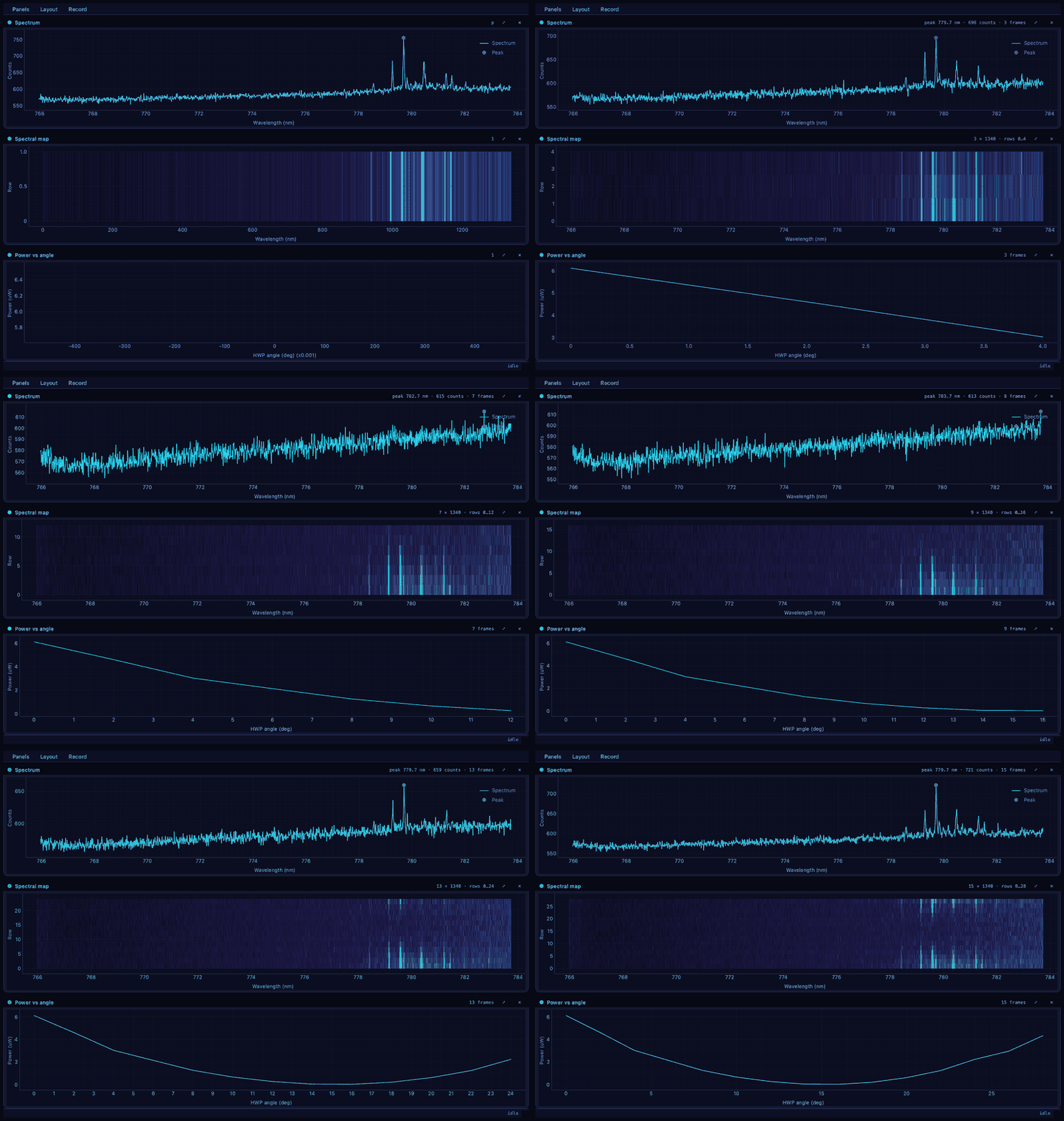
Three views of one measurement, updating together: the newest spectrum, every spectrum so far stacked into a map, and the power curve. They are reading the same records.jsonl the single-panel window read in lesson 5 — nothing was added to the experiment to make this possible, and nothing can be broken in the experiment by watching it.

Two subcommands are worth knowing before you need them:

uv run python -m plesty.demo_pol_pl.viz monitor --replay 2   # a stored run, 2 rows a tick
uv run python -m plesty.demo_pol_pl.viz monitor --run <id>   # a particular run, live or not

--replay is how you show someone a measurement that finished last night at the pace it happened, and it is the same window, the same panels, the same monitors. A monitor that accumulated its curve in the renderer instead of in update would not survive this; yours do.

Render it without a screen

The last subcommand needs no window at all:

uv run python -m plesty.demo_pol_pl.viz render --run demo_pol_pl_20260821-221323

[viz] rendering demo_pol_pl_20260821-221323 → …/demo_pol_pl_20260821-221323.mp4
[viz] saved …/demo_pol_pl_20260821-221323.mp4

Qt runs offscreen, the shell draws into an image buffer, and the run is encoded a frame per tick. It writes MP4 when imageio-ffmpeg is installed — that is what the record extra brought — and falls back to an animated GIF when it is not, in which case the saved name is not the one it announced.

This is how a measurement gets into a group meeting, and it is worth knowing that it runs on a headless machine: render on the acquisition PC over SSH, at three in the morning, is a normal thing to do.

When a view outgrows your experiment

Your three monitors name this bench — HWP angle (deg) on an axis, hwp_deg in a mapper — which is right for a first version. The ideas under them are not specific at all, and plesty-common-monitors is where the general forms live:

Take MalusMonitor. Strip the names off it and it is two lists, a point appended per row, and a line through them — which is SeriesMonitor:

So the whole of lesson 5 is also this, with no class of your own:

from plesty.common_monitors import SeriesMonitor, series_mapper
from plesty.lib.monitor import RunSource

monitor = SeriesMonitor(
    RunSource(run_dir, mapper=series_mapper("hwp_deg", "power_w", y_scale=1e6)),
    x_label="HWP angle (deg)",
    y_label="Power (uW)",
)

Same 91 rows, same curve — the trace is called series rather than malus, and that is the only difference you would notice.

Which answers what was ever specific to your experiment: not the monitors, the mapper. Look in the shared package before writing a view, and lift your own into it when a second experiment asks for it — not before, since generality invented up front is guesswork.

Next

That is the last lesson. The wrap-up is what the six of them add up to, and what changes when the instruments are real ones — the short answer being: the configuration, and none of the code.